Maze Solver Robot Simulator for Flood-Fill Planning

Controls

Pick a mode — Explore, then speed-run or Speed-run only — and press Start to watch it solve, or Step one move at a time. New maze builds a fresh random maze; Reset replays the same one. Three speeds, keyboard shortcuts, and Full screen keep the run controllable. Bold lines are the maze walls, the shaded corridors are everywhere the robot explored (dead ends included), and the bold line is the shortest path flood fill found.

Theory

A grid maze is cells joined by open edges, with walls between the rest. To find the shortest route a robot must first know the maze — so this lab runs two phases.

Explore. The robot walks the maze depth-first with a left-hand rule: at each junction it turns left if it can, otherwise straight, then right. When it hits a dead end it backtracks to the last junction and takes the next branch. Repeating that until every cell is visited maps the whole maze — including all the wrong paths it had to rule out.

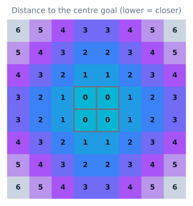
Optimise. With the map complete, a flood fill assigns the goal a distance of zero and propagates increasing values outward through every open edge. Every cell now holds its distance to the goal, so the shortest path is simply this: from the start, always step to a neighbour one number lower. The robot speed-runs that path — far shorter than the wandering exploration.

Algorithm

1. Explore the maze depth-first with a left-hand rule, backtracking out of every dead end, until all cells are visited.
2. Record each open edge on both sides so the finished map knows every wall.
3. Flood-fill from the goal: label it 0 and propagate increasing distances outward through every open edge.
4. Read the shortest path off the field: from the start, repeatedly step to a neighbour whose distance is one lower.
5. Speed-run that path to the goal.
6. Compare the exploration length with the shortest-path length to see how much wandering the map saved.

Source code

Keep exploration, mapping, planning, and motion as separate functions:

// Phase 1 — map the whole maze, backtracking out of dead ends
exploreDepthFirst(map, robot);        // left-hand rule until every cell is visited

// Phase 2 — flood-fill the finished map and run the shortest path
map.floodFill(goal);                  // goal = 0, distances ripple outward
for (Cell c = start; c != goal; c = map.lowerNeighbor(c))
  robot.driveTo(c);                   // always step one distance lower

That boundary makes the same planner testable in this browser lab, on a desktop, and on the final ESP32 controller.

Assumptions and hardware differences

The lab makes mapping clean by removing the hard part of a real Micromouse: odometry. The simulated robot moves exactly one cell per step with no wheel slip, no gyro bias and no 90° turn error, and its three range sensors report walls perfectly with no false positives. A physical ESP32 build accumulates heading and distance error every move, must re-square against walls, and must filter ToF readings against sunlight and supply sag — which is why the precise turns tutorial and the flood-fill guide spend more time on motion than on planning. Use this simulator to learn why flood fill replans, not to prove your motion layer.

Circuit diagram

Use an external regulator sized for the motor stall current. The ESP32 and sensors need a stable logic rail even when motors reverse.