Lidar for Robots: What a Scan Gives You and How It Becomes a Map

Introduction

A distance sensor tells you how far away one thing is, along one line. A map tells you the shape of a room. Everything interesting in navigation lives in the gap between those two, and that gap is what this page is about.

The two ends are already covered here: single-point ranging on one side, and SLAM and A* over an occupancy grid on the other. But those assume a grid already exists. Nothing says where it came from, and the answer — ray casting a scan into cells — is both simple and full of traps.

A 2D lidar is a ToF sensor on a turntable

This is the most useful thing to know, because it means you already understand the ranging half.

Inside a hobby 2D lidar there is one optical time-of-flight ranging module, exactly the kind on a VL53-series breakout, pointed sideways and spun. An angular encoder reports where it was looking at each measurement. Power and data cross the rotating boundary through a slip ring or an optical/inductive coupling.

So a “scan” is not a photograph. It is a list of (angle, range) pairs, gathered one at a time, over one revolution. Every limitation below follows from that sentence.

This also tells you why ultrasonic sensors do not get spun into lidars. An ultrasonic beam is tens of degrees wide, so rotating it gains you almost nothing — you would be smearing an already-wide beam across the room. A narrow optical beam is what makes angular resolution meaningful in the first place. Sweeping a single ToF sensor on a servo, as in the scanning ultrasonic tutorial, really is a slow, low-resolution lidar.

The sample budget is fixed, so resolution and freshness trade

Here is the part that surprises people, and it is worth understanding before you buy anything.

The ranging module has one throughput number: how many measurements per second it can take. On an RPLIDAR A1 that is about 8000 samples per second, and it does not change when you change the spin rate. The spin rate is yours to choose, typically 1–10 Hz.

So the points you get per revolution are simply the budget divided by the spin rate:

points per revolution = samples per second ÷ spin rate
angular step          = 360° ÷ points per revolution

Spin rate	Points per revolution	Angular step	Scan period
5.5 Hz	1455	0.25°	182 ms
10 Hz	800	0.45°	100 ms

You cannot have fresh scans and fine angular resolution at the same time. Spinning at 10 Hz halves your latency and nearly halves your angular resolution. That single trade decides more about how a robot behaves than the headline range figure does, and it is the first thing to set deliberately rather than leave at whatever the driver defaults to.

Fast-moving robot in an open corridor: spin fast, you need the freshness and the walls are big. Slow robot mapping a cluttered room: spin slowly, you need the detail and you can afford the latency.

Beams diverge, so distant obstacles fall between them

An angular step is an angle, not a distance. Two adjacent beams separate as they travel:

gap between beams ≈ range × angular step (in radians)

At 0.45° that is 7.9 mm of gap at one metre, and 31 mm at four metres. Nothing samples the space in between.

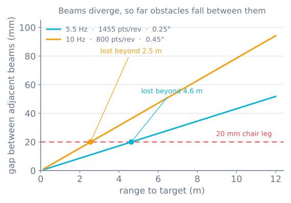
Take a 20 mm chair leg. Spinning at 10 Hz, the beam gap passes 20 mm at about 2.5 m — beyond that the leg can sit entirely between two beams and return nothing. At 5.5 Hz you get to about 4.6 m before the same thing happens.

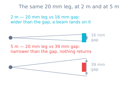
This explains a behaviour that otherwise looks like a broken sensor: thin obstacles appear as the robot approaches, popping into the map a metre or two out. The lidar was not failing. The leg was never sampled.

Two consequences worth designing around:

• Do not trust a single scan for thin obstacles. Accumulating several scans into a grid, as below, is what actually finds table legs — each scan samples slightly different angles.
• Chair and table legs are the classic domestic robot failure, because they are thin, they are at exactly lidar height, and the robot only learns about them late.

A scan is not a snapshot

The points in one revolution were not measured at the same instant. At 5.5 Hz the sweep takes 182 ms, and the robot does not politely wait.

• Driving at 0.5 m/s, the robot travels 91 mm during one revolution.
• Turning at 1 rad/s, the scan is smeared through 10.4°.

Treating that list of points as one rigid snapshot taken at one pose bends the world. Straight walls come out curved or doubled, and scan matching fights corrections that are really your own motion.

This is why sensor_msgs/LaserScan carries scan_time and time_increment alongside the ranges: they let a consumer work out when each beam was taken. Correcting for it — transforming each point by the pose the robot held at that beam’s timestamp — is called deskewing or motion compensation, and good SLAM front ends do it for you.

What this means practically: if your maps are clean while stationary and smeared while moving, suspect deskewing and timestamps long before you suspect the sensor. And slow down while mapping. Half the speed is half the distortion, for free.

One horizontal slice is all you get

A 2D lidar measures a plane. Whatever sits above or below that plane does not exist.

The classic three:

• Overhangs. A table top at 700 mm is invisible to a lidar at 150 mm. The robot drives confidently underneath and wedges itself.
• Low obstacles. A door threshold, a cable, a sock. All below the plane.
• Drop-offs. A descending stair is empty space in every direction the lidar can see. It reads as beautifully clear floor.

No amount of scan processing fixes this, because the information was never captured. Real robots keep a bumper, cliff sensors and often a downward or forward-tilted ranger alongside the lidar — not because the lidar is bad, but because a plane is a plane. When you read that a vacuum robot “has lidar and still has bumpers”, this is why.

From scan to grid: ray casting

Now the mapping half. An occupancy grid divides the world into square cells and stores, for each one, how strongly you believe it is occupied.

The insight that makes it work: a range reading tells you about every cell along the ray, not just the cell at the end. If a beam travelled 3 m before hitting something, then all the space it crossed must have been empty — otherwise it would have stopped sooner.

So each beam produces three verdicts:

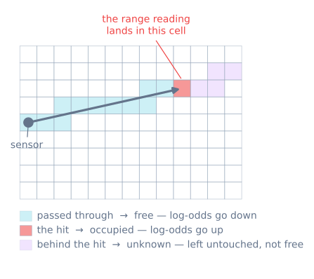
1. Cells the ray passed through → evidence of free. Walk the line from sensor to hit and nudge each cell towards empty.
2. The cell the reading landed in → evidence of occupied. Nudge it towards full.
3. Cells beyond the hit → nothing. The beam stopped. You learned nothing about what is behind that wall, so you must leave those cells alone.

Walking the line is just line rasterisation — Bresenham’s algorithm, the same one that draws a line on a screen.

A max-range reading needs its own handling. Many drivers report the maximum, or infinity, when nothing came back. That is not “there is a wall at 12 m” — it is “nothing was found”. Mark the ray free and mark no occupied cell at the end.

Log-odds: why you add instead of multiply

You could store a probability per cell and multiply Bayes updates together. In practice everyone stores log-odds instead:

l = ln( p / (1 - p) )          p = 1 / (1 + e^(-l) )

Two reasons. Multiplying many small probabilities underflows; adding logs does not. And it makes the update a single addition, which is cheap enough to do for every cell of every beam of every scan.

With p = 0.5 (no idea) mapping to l = 0, pick one value for a hit and one for a miss — say p_occ = 0.7 (l = +0.847) and p_free = 0.4 (l = −0.405) — and the update is:

l_cell += l_occ     # this beam hit this cell
l_cell -= 0.405     # this beam passed through this cell

A cell starting at l = 0 after three hits:

Observation	Log-odds	Probability
start (unknown)	0.000	0.500
hit	+0.847	0.700
hit	+1.695	0.845
hit	+2.542	0.927
passed through	+2.136	0.894
passed through	+1.731	0.850

Evidence accumulates, and disagreement pulls it back. That is the whole algorithm.

Clamp the totals. This matters more than it looks. Twenty consecutive hits without a clamp put a cell at l = 16.9, which is p = 0.999999. Now someone moves the chair. Undoing that certainty takes 42 free observations. The chair leaves a permanent phantom, and your planner keeps steering around nothing.

Clamping l to something like ±3.5 fixes it: strong belief is still strong, but a handful of contradicting scans can overturn it. If your maps accumulate ghosts of objects that have gone, this is almost always why.

Unknown is a third state, not a synonym for free

This is the mistake that produces confident, dangerous plans.

A freshly initialised grid is entirely unknown. If your planner treats unknown as traversable, it will happily route straight through the parts of the world you have never looked at — and being unexplored, they are exactly where the surprises live. If it treats unknown as blocked, the robot refuses to move at the start, because everything is unknown.

Both are wrong; keep the three states distinct and decide deliberately:

• Occupied — do not plan through it.
• Free — plan through it.
• Unknown — plan through it only at a cost, or only when deliberately exploring.

Frontier exploration, which is how a robot chooses where to look next, is built entirely on the free/unknown boundary. Collapse the two and you have thrown that away.

Choosing cell size

The usual answer is 5 cm for indoor robots, and there is a reason not to go finer just because you can.

A cell smaller than your beam spacing at typical range is inventing precision you do not have — at 4 m the beams are 31 mm apart, so 1 cm cells leave permanent holes between rays that never fill in. Cells much larger than your robot’s clearance margin, meanwhile, make doorways look impassable, because a single occupied cell can swallow the gap.

Practical rule: cell size a little smaller than the narrowest gap you must drive through, and no smaller than your beam spacing where you actually operate. Then inflate obstacles by the robot radius at planning time rather than shrinking cells to compensate.

When it goes wrong

Symptom	Usually
Thin obstacles appear only when close	Beam spacing exceeded their width at range — expected, not a fault
Walls curve or double while driving	Scan not deskewed; points treated as one instant
Map clean when still, smeared when moving	Same cause; also try mapping slower
Robot drives under a table and wedges	2D plane cannot see overhangs; needs a second sensor
Stairs read as open floor	Drop-offs are invisible to a horizontal plane; cliff sensors
Obstacles that were removed stay on the map	Log-odds not clamped, so certainty cannot be undone
Whole map fills with obstacles at the edges	Max-range “no return” readings marked as hits
Planner routes through unexplored space	Unknown conflated with free
Fine grid full of speckle holes	Cells smaller than beam spacing; nothing samples between rays
Glass walls missing entirely	Optical returns pass straight through — the one place ultrasonic wins

That last row is the honest caveat for the whole page. Lidar beats sonar on resolution, rate and range, and then loses completely to it on a glass door, which sound reflects off and light does not. It is the clearest argument for not choosing one sensor and calling the problem solved.