Motion Profiles: Trapezoidal and S-Curve Acceleration

Introduction

Tell a motor to go to a position and it will try to get there immediately. Not quickly — immediately. The command contains no information about how fast, so the only interpretation available is “as fast as possible”, and what happens next is decided by whatever runs out first: torque, current limit, traction, or the stepper’s ability to keep up.

A motion profile is the missing information. It turns “go to 100 mm” into a schedule — where should the axis be at every instant between now and arrival — and hands the controller a target that moves at a speed the machine can actually deliver.

This is the difference between a robot arm that arrives and one that arrives and stops shaking.

What a bare position command actually asks for

Consider a step: at t = 0 the target jumps from 0 mm to 100 mm.

To follow that exactly, the axis would need infinite velocity, which requires infinite acceleration, which requires infinite force. It cannot, so something gives:

• A stepper is commanded to a step rate its torque cannot produce at that speed, misses steps, and — running open loop — has no idea it did. Position is now permanently wrong.
• A DC motor with a PID loop sees an enormous instantaneous error, saturates its output, winds up its integral term, and overshoots.
• A servo slams to its maximum rate and arrives with the whole mechanism still moving.

None of these are tuning problems. They are all the same problem: the command was physically impossible.

The trapezoidal profile

The fix is to command velocity, and to change velocity at a rate the motor can sustain. Accelerate at a constant rate to a cruise speed, hold it, then decelerate at the same rate. Plot velocity against time and it is a trapezoid, which is where the name comes from.

Three numbers define it: the distance d, a top speed v_max, and an acceleration a.

t_accel = v_max / a                     time spent ramping
d_accel = v_max² / (2a)                 distance used by one ramp
t_total = v_max / a  +  d / v_max       whole move, if it reaches v_max

For a 100 mm move at 100 mm/s with a = 500 mm/s²: each ramp takes 0.2 s and covers 10 mm, leaving 80 mm of cruise, for a total of 1.2 s.

Here is the whole thing as a function of time — the position your control loop should be chasing at instant t:

// Target position t seconds into a trapezoidal move of `d` mm.
float profilePosition(float t, float d, float vMax, float a) {
  float tAcc = vMax / a;
  float dAcc = vMax * vMax / (2 * a);

  if (2 * dAcc > d) {                      // too short to reach vMax
    float tPeak = sqrtf(d / a);            // triangular profile
    if (t >= 2 * tPeak) return d;
    if (t < tPeak) return 0.5f * a * t * t;
    float left = 2 * tPeak - t;
    return d - 0.5f * a * left * left;
  }

  float tCruise = (d - 2 * dAcc) / vMax;
  float tTotal  = 2 * tAcc + tCruise;
  if (t >= tTotal) return d;
  if (t < tAcc)           return 0.5f * a * t * t;
  if (t < tAcc + tCruise) return dAcc + vMax * (t - tAcc);

  float left = tTotal - t;
  return d - 0.5f * a * left * left;
}

Note what this function is not: it is not a controller. It generates a setpoint. Whatever you had — a stepper step scheduler, a PID loop, a servo write — still does the following. The profile only changes what it is following.

The move you asked for is not always the move you get

That 2 * dAcc > d branch is the case people meet first and misdiagnose.

If the move is shorter than the distance needed to accelerate up and back down again, the axis never reaches the speed you configured. It ramps up, hits the halfway point, and immediately ramps down — a triangle, not a trapezoid.

The threshold is d < v_max² / a. For the numbers above that is 20 mm, so every move shorter than 20 mm tops out below 100 mm/s no matter what you set.

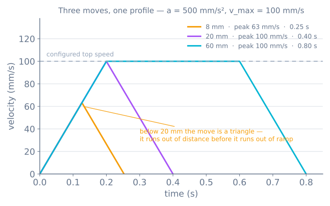
This is why raising v_max on a machine that does lots of short moves changes nothing measurable. The moves were never speed-limited; they were acceleration-limited. A 3D printer doing dense infill is the everyday example.

The corners are still discontinuous

The trapezoidal profile fixed velocity. Look at acceleration and the problem has simply moved.

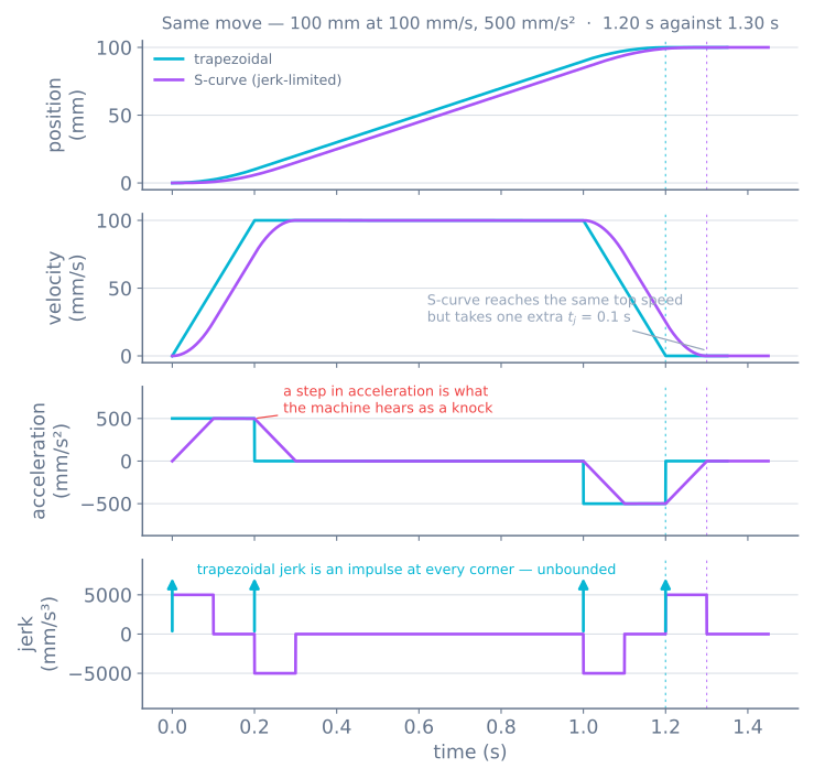
At t = 0 acceleration jumps from 0 to 500 mm/s² instantly. At the top of the ramp it drops back to 0 instantly. Each of those is a step in acceleration — and the rate of change of acceleration is jerk, so a step in acceleration is an infinite jerk impulse.

Infinite is not a number a machine can produce either. What it produces instead:

• An audible knock at the start and end of every ramp.
• Ringing — belts stretch, couplings wind up, and the structure has compliance, so a sudden force change excites it and it oscillates afterwards. On a printer this is the ghosting you see beside sharp features.
• Torque spikes that trip current limits which the average torque figure said were fine.

The S-curve

An S-curve profile limits jerk as well as acceleration. Instead of stepping to full acceleration, it ramps into it over a jerk time t_j = a_max / j_max, holds, then ramps out. The velocity curve gains rounded corners — hence the name — and acceleration becomes a trapezoid of its own.

A full S-curve move has seven phases: jerk up, hold acceleration, jerk down, cruise, and the mirror image to stop.

What it costs: exactly one t_j

This is the part worth committing to memory, because it makes the trade concrete.

When both profiles reach the same v_max and the same a_max, the S-curve move takes longer by exactly t_j — one jerk time, not two, and regardless of how far the move is:

trapezoidal   T = v_max/a + d/v_max
S-curve       T = v_max/a + d/v_max + t_j          where t_j = a_max / j_max

For the worked move: 1.2 s becomes 1.3 s. An 8% penalty on this move, and a smaller percentage on longer ones, in exchange for bounded jerk.

The reason it is one and not two: the S-curve’s acceleration segment is longer, so it covers more distance before cruising, so the cruise phase shrinks and gives most of the time back. Only the jerk time itself is unrecoverable.

There is a constraint hiding in there. The acceleration only reaches a_max if v_max ≥ a_max² / j_max. Below that the move never reaches full acceleration either, and you get a triangular acceleration profile — the same “ran out of distance” story, one derivative up.

“Jerk” in printer firmware is not jerk

Worth knowing before you go tuning anything, because the vocabulary actively misleads.

Classic Marlin’s DEFAULT_XJERK is not the derivative of acceleration. It is the maximum instantaneous velocity change permitted at a junction between two moves, in mm/s — a cornering allowance that lets the planner take a corner without decelerating to zero. Useful, but a different quantity with the wrong name and the wrong units.

Newer Marlin defaults to Junction Deviation instead, which models the corner as a circular arc of a given deviation in mm. Klipper uses square_corner_velocity — the speed at which a 90° corner is taken. All three are answers to “how do I not stop at every corner?”, and none of them is a jerk limit in the physics sense.

So if a forum post tells you to lower your jerk to stop ringing, check which quantity is meant. Lowering junction velocity reduces cornering shock; it does not bound da/dt within a single move.

Your PID is probably fine

If you have a closed-loop axis that overshoots and oscillates on every move, the instinct is to detune it — drop Kp, add derivative, fight the overshoot.

Try profiling the setpoint first.

A step input asks a PID controller for infinite output. Its error term starts at the full move distance, the derivative term sees an instantaneous jump, and the integral term accumulates while the output is saturated and the axis cannot respond. Detuning makes the controller sluggish everywhere in order to survive one impossible instant.

With a profile, the error stays small for the entire move, because the target is somewhere the axis can actually be. The same gains that were unusable against a step are often well-behaved against a ramp — and now the controller is only correcting for load and friction, which is what it is for. You can watch the difference in the PID simulator by comparing a step setpoint against a gradual one.

Where you meet this on a real robot

• Steppers. AccelStepper’s setMaxSpeed() and setAcceleration() give you a trapezoidal profile and nothing else. There is no S-curve option; for that you generate the setpoint yourself.
• Hobby servos. An SG90 has an internal controller you cannot see or tune, so profiling means stepping the commanded angle gradually instead of writing the target in one call — the same idea applied from outside.
• DC motors with encoders. Profile the position setpoint and let the encoder PID follow it. This is the arrangement where profiling pays best.
• Mobile robots. The same limit applies to linear.x on a cmd_vel bridge: commanding a velocity step makes the wheels slip, which corrupts odometry. Rate-limit the twist.
• Printers and CNC. Marlin, Klipper and GRBL all plan trapezoidal moves with a cornering rule between them.

When it goes wrong

Symptom	Usually
Stepper loses position under load, silently	No profile — commanded rate exceeds pull-in torque
Machine knocks at the start and end of moves	Trapezoidal jerk impulse; needs S-curve or lower acceleration
Ringing beside sharp features	Structural resonance excited by acceleration steps
Short moves ignore the speed setting	Triangular profile — acceleration-limited, not speed-limited
Overshoot and oscillation on every move	Step setpoint into a closed loop; profile it before detuning
Raising acceleration helps, then suddenly does not	Now torque-limited rather than profile-limited
Odometry drifts badly during starts	Wheel slip from a velocity step; rate-limit the command

Profiling is the cheapest large improvement available to most hobby motion systems, because it costs one function and no hardware. The robot arm simulator is a good place to see why it matters at the end of a long link, where a small acceleration step at the base becomes a visible wobble at the gripper.